Functions to Plot Results From cvSim
When we use the function cvSim to create an object it returns to the object a list that contains the following vectors and matrices
time: a vector that contains the discrete times used to define the diffusion griddistance: a vector that contains the discrete distances used to define the diffusion gridpotential: a vector that contains the discrete applied potentials corresponding to the discrete times used in the simulationcurrent: a vector that contains the calculated current at each discrete applied potentialoxdata: a matrix that contains the concentrations of the oxidized species in the diffusion grid; each row in the matrix is a discrete time and each column in the matrix is a discrete distancereddata: a matrix that contains red concentrations of the reduced species in diffusion grid; each row in the matrix is a discrete time and each column in the matrix is a discrete distanceormalE: the redox couple’s formal potential
We can access this data to display the results of a simulation in a variety of useful ways. All the functions described here are included in the document CV Functions.
Plotting the Cyclic Voltammogram
To plot the cyclic voltammogram, we use the plotCV function
plotCV(file, overlay = FALSE)which takes the inputs shown in parentheses where file is the name of the object created by cvSim and overlay allows for plotting more than one CV on the same set of axes (note: the default option of FALSE draws the axes and the CV; setting overlay to TRUE plots the CV only). In addition to the cyclic voltammogram, the resulting output includes a vertical dashed line at the redox couple’s formal potential and a horizontal dashed line at a current of zero. The following code shows how to overlay the results of two simulations:
# first, plot the results for testCV2
plotCV(testCV2)
# and then overlay the results for testCV1
plotCV(testCV1, overlay = TRUE)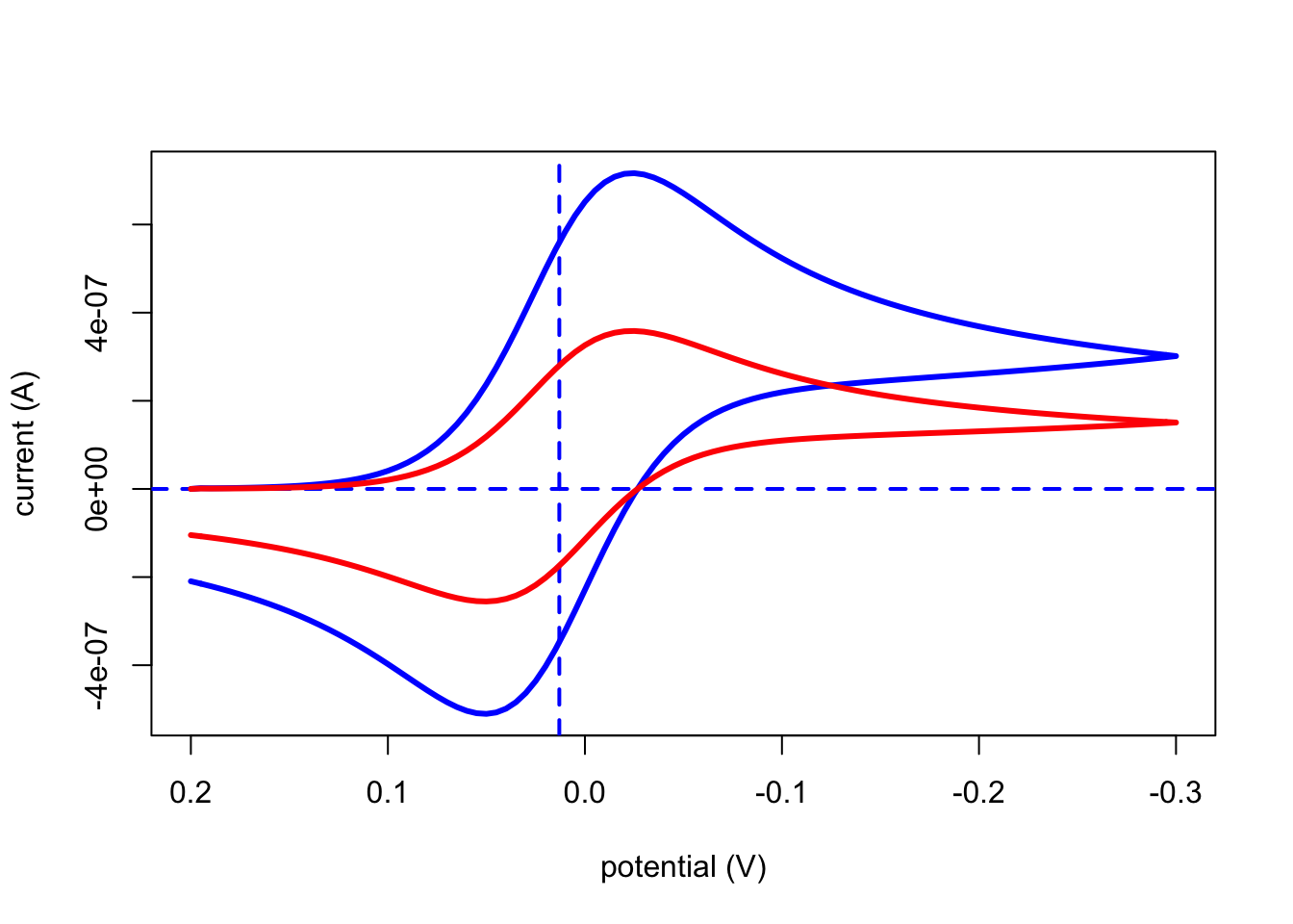
We also can plot the cyclic voltammogram using the plotly library using the function
plotlyCV(file)which takes as its only input the name of the object created by cvSim. The resulting output provides an interactive plot; move your cursor inside the plot to explore the possibilities.
plotlyCV(testCV1)Plotting the Applied Potential Waveform
To plot the applied potential waveform, we use the plotPotential function
plotPotential(file)which takes as its only input the name of the object created by cvSim. The resulting output is self-explanatory.
plotPotential(testCV1)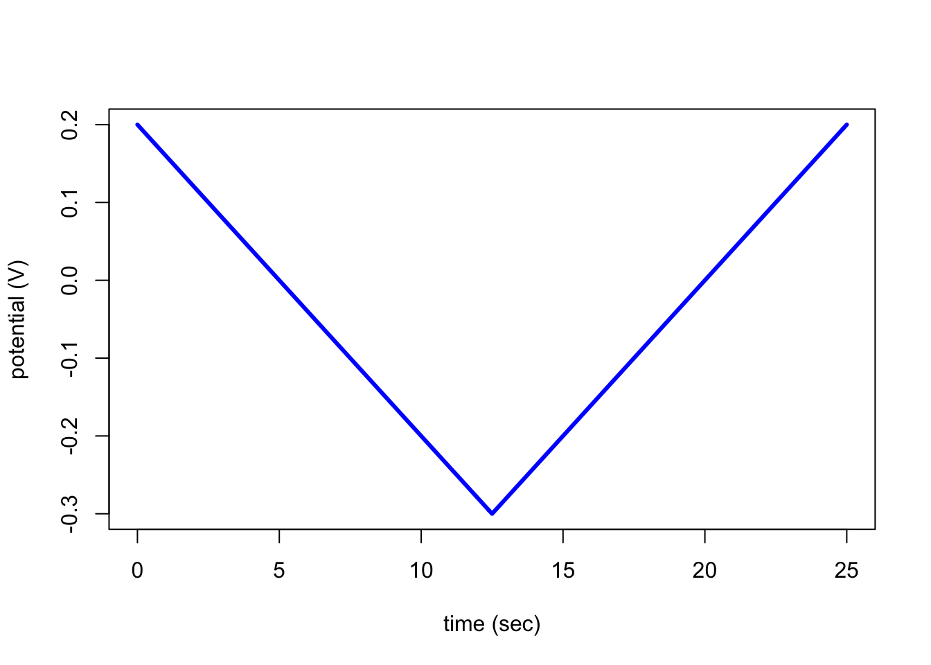
Ploting the Diffusion Profile at a Specific Time
A diffusion profile shows how the concentrations of the redox couple’s oxidized and reduced forms change as a function of distance from the electrode surface at a particular time during cyclic voltammogram. To plot the diffusion profile, we use the plotDiffusion function
plotDiffusion(file, index = 1, both_species = TRUE) which takes the inputs shown in parentheses where file is the name of the object created by cvSim, index is used to specify the time (for example, index = 1 is the first time unit), and both_species plots the diffusion profile for both the analyte’s oxidized and its reduced forms (note: the default option of TRUE includes both; setting both_speices to FALSE plots the diffusion profile for the analyte’s oxidized form only). The resulting output displays the concentration of the redox couple’s oxidized form in blue and the concentration of its reduced form in red.
# let's examine the diffusion profile for the 100th point in simulation
plotDiffusion(testCV1, index = 100)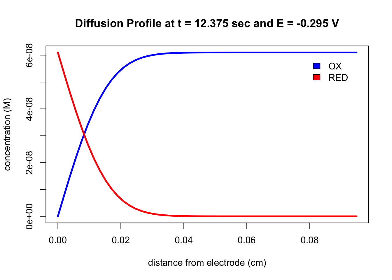
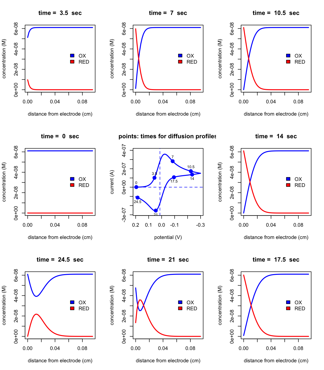
Plotting a Grid of Diffusion Profiles
The function plotGrid produces a 3 \(\times\) 3 grid of plots showing, at the grid’s center, a cyclic voltammogram, and, arranged around the CV, eight diffusion profiles equally spaced in time. The function takes the form
plotGrid(file)which takes as its only input the name of the object created by cvSim. The following plot shows typical example.
plotGrid(testCV1)