Three Important Concepts
Suppose you have an electrode sitting in a solution that is 1.0 \(\times\) 10-6 M Fe3+ and 0 M in Fe2+. To understand what happens when you apply an initial potential to the electrode, or what happens if you change the applied potential, you must understand three important and interrelated concepts:
- that the electrode’s potential determines whether the analyte is present at its surface as Fe3+, as Fe2+, or as a combination of both Fe3+ and Fe2+
- that the concentration of Fe3+ (and, for that matter, Fe2+) at the electrode’s surface may not be the same as its concentration in bulk solution
- that the current flowing at the electrode is a measure of the rate at which the Fe3+ is reduced to Fe2+ or the rate at which Fe2+ is oxidized to Fe3+
To help you think through these concepts, the following sections will present you with some data and some questions to consider. You may add your answers to these questions, as well as any additional questions or thoughts that you have. When done, save and knit the file to update this file’s contents.
You may wish to review the paper “Understanding Electrochemistry: Some Distinctive Concepts”, the full citation for which is Faulkner, L. R. J. Chem. Educ. 1983, 60, 262–264 (DOI). In addition to the three important concepts you will explore here, this paper also presents two additional important concepts that are explored in another short read.
The Applied Potential Determines the Analyte’s Form at the Electrode’s Surface
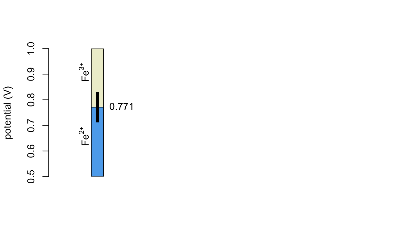
The figure below is a ladder diagram for the Fe3+/Fe2+ redox couple. You may recall that a ladder diagram provides information about the relationship between the applied potential and the oxidized and reduced form of the analyte.
Questions to Consider
What is the significance of each of the following features of this ladder diagram: (a) the value 0.771, (b) the area shaded in blue, (c) the area shaded in light yellow, and (d) the vertical black bar?
Based on this ladder diagram, what form(s) of iron are present at the electrode’s surface when the applied potential is 1.00 V? is 0.80 V? is 0.75 V? is 0.60 V?
The Analyte Can Have Different Concentrations at the Electrode and in Solution
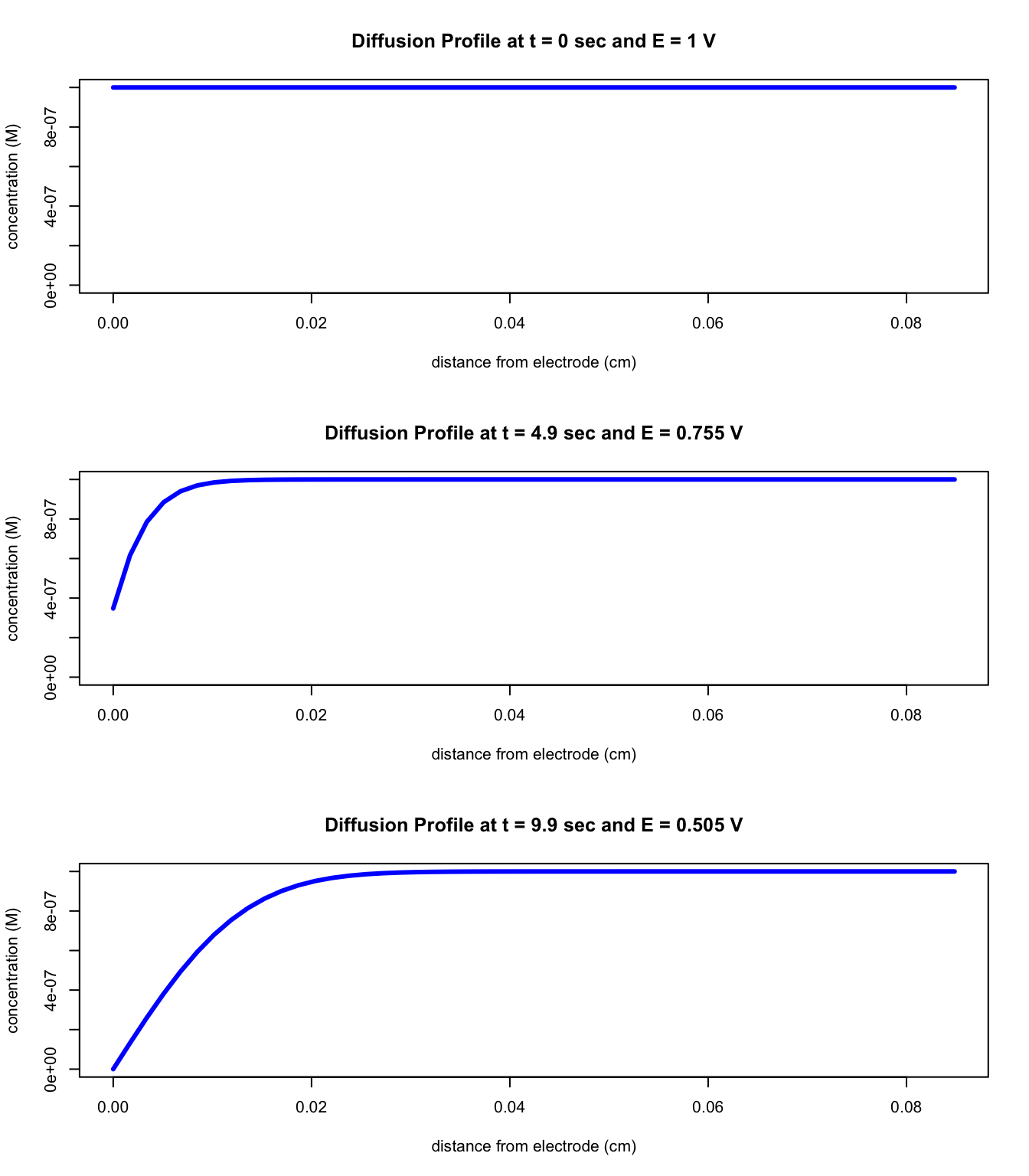
Suppose you have a solution that is 1.0 \(\times\) 10-6 M in Fe3+ in contact with an electrode with an applied potential of 1.0 V and that you scan the potential toward 0.5 V at a scan rate of 0.05 V/s. The figures below show the concentration of Fe3+ as a function of distance from the electrode surface (we call this plot a diffusion profile) at a potential of 1 V, at a potential of 0.755 V, and at a potential of 0.505 V.
Questions to Consider
Why do you think these diagrams are called diffusion profiles?
For each of the three figures, explain the shape of the curve paying particular attention to differences in the concentration of Fe3+ at the electrode surface and difference in the distance from the electrode surface at which the concentration of Fe3+ is equal to that in bulk solution.
The Nernst equation for the Fe3+/Fe2+ redox couple is
\[ E = E^{o}_{\textrm{Fe}^{3+}/\textrm{Fe}^{2+}} - 0.05916\log { \frac { \left[\textrm{Fe}^{2+}\right] }{ \left[\textrm{Fe}^{3+}\right] } } \]
Given the applied potentials and knowing that the total concentration of Fe3+ and of Fe2+ at the electrode surface must equal the initial concentration of Fe3+ (why?), calculate the concentration of each species at the electrode surface. Are your results in agreement with the figure above?
Current is a Measure of the Rate of Oxidation or the Rate of Reduction at the Electrode’s Surface
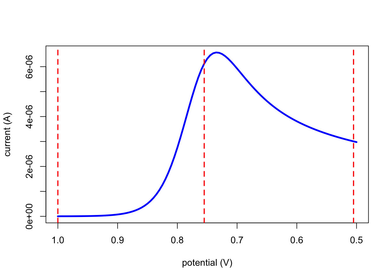
The figure below shows how the current changes as we scan the potential from 1.0 V to 0.50 V at a scan rate of 0.05 V/s under the same conditions as in the previous section; the vertical dashed lines show the three potentials considered in the previous section.
Questions to Ponder
Explain why you can express the rate at which Fe3+ is reduced to Fe2+ using the following equation
\[ \textrm{rate} = \frac { \Delta \left[ \textrm{Fe}^{3+} \right] }{ \Delta t } \]
Given this equation, and drawing on your responses to the questions in the previous section, explain the general shape of the plot of current as a function of potential.
Extending Your Analysis
At this point you should have a working understanding of these three important concepts
- that the electrode’s potential determines whether the analyte is present at its surface as Fe3+, as Fe2+, or as a combination of both Fe3+ and Fe2+
- that the concentration of Fe3+ (and, for that matter, Fe2+) at the electrode’s surface may not be the same as its concentration in bulk solution
- that the current flowing at the electrode is a measure of the rate at which the Fe3+ is reduced to Fe2+ or the rate at which Fe2+ is oxidized to Fe3+
The figure below shows results for a cyclic voltammetry experiment for this same system involving the Fe3+/Fe2+ redox couple. For this experiment, the potential is scanned from 1.0 V to 0.50 V at a rate of 0.05 V/s and then the potential immediately is scanned back to 1.0 V at the same rate.
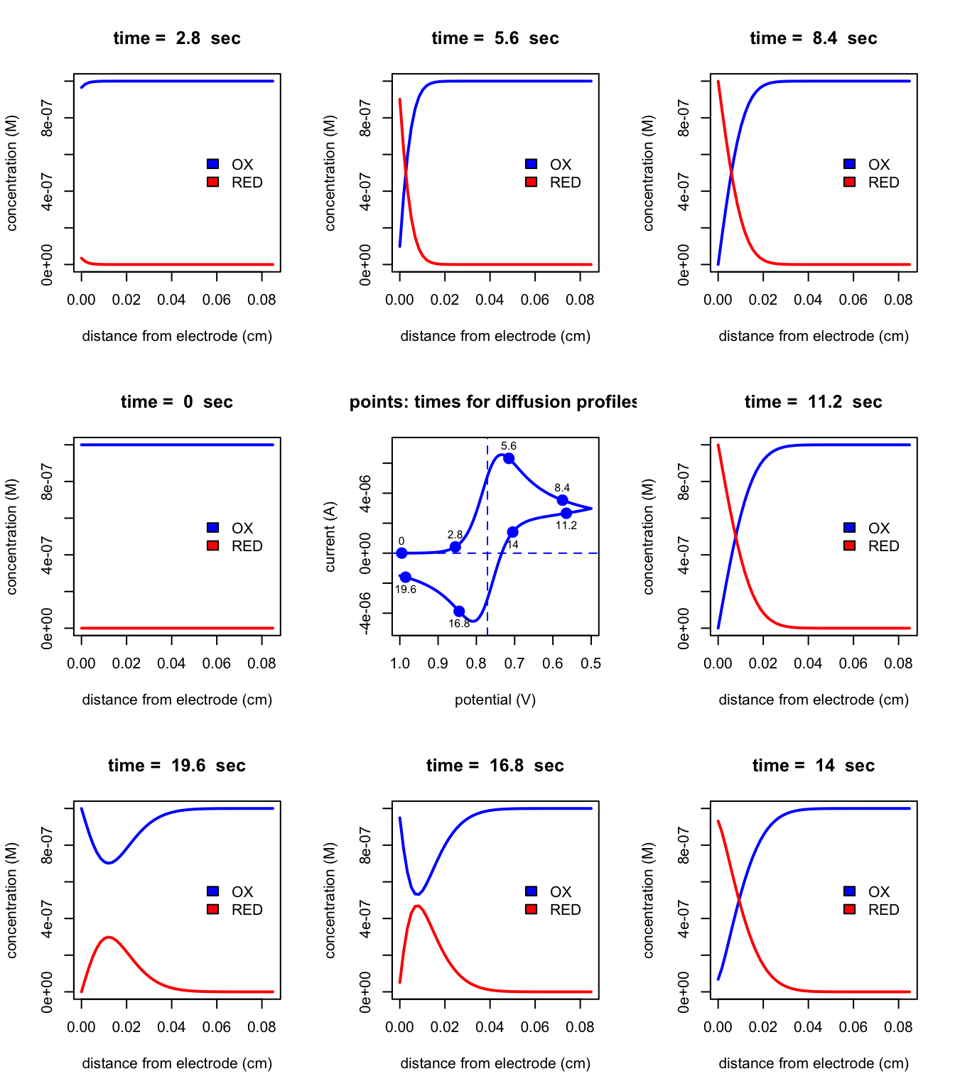
The figure at the center of the grid shows how the current changes as a function of the applied potential—this is called a cyclic voltammogram—and the remaining figures show concentration profiles for Fe3+ and for Fe2+ at different times (and thus different applied potentials). The two dashed lines on the central figure show the redox couple’s formal potential and a current of 0 A. Using what you have learned in this short read, explain the shape of the eight diffusion profiles (paying particular attention to those at times of 16.8 and of 19.6 s) and the shape of the cyclic voltammogram.